Introducing the Zymtrace GPU Execution Timeline
Zymtrace now records individual kernel, memory-copy, and synchronization events with nanosecond timestamps, full CPU launch stacks, and a GPU memory overlay.


Tim Denk
Zymtrace now has a GPU execution timeline. It records individual kernel, memory-copy, and synchronization events with nanosecond timestamps, full CPU launch stacks, and a GPU memory overlay. Profiling can be enabled on running processes from the UI without a restart, and coding agents can analyze execution patterns, durations, and gaps through MCP.
Investigating GPU performance often means tracing delays between kernel launches, memory transfers, and synchronization points. Serialized copies, launch gaps, and inconsistent batch execution can limit throughput even after the expensive kernels have been optimized.
The timeline is built for exactly those questions. It preserves event order, overlap, and gaps, complementing the aggregated view of the AI flamegraph; see the appendix for guidance on which view to use. Large traces load incrementally, and microsecond kernels stay visible even when zoomed out.
On a sentence-transformers workload, the timeline and profiling data guided four changes that reduced run time from 568s to 82s.
Enable high-resolution profiling on demand
Enable high-resolution profiling from the Zymtrace UI without restarting your workload. Select workloads and a duration to capture every GPU event, rather than the samples collected by always-on profiling.
The selection is a rule in the agent configuration, so profiling can be scoped to specific projects, hosts, and processes, with each session capped at 10 minutes. That makes it practical to investigate the workload’s current request mix, batching behavior, and memory pressure instead of arranging a separate profiling run against a reconstructed setup.
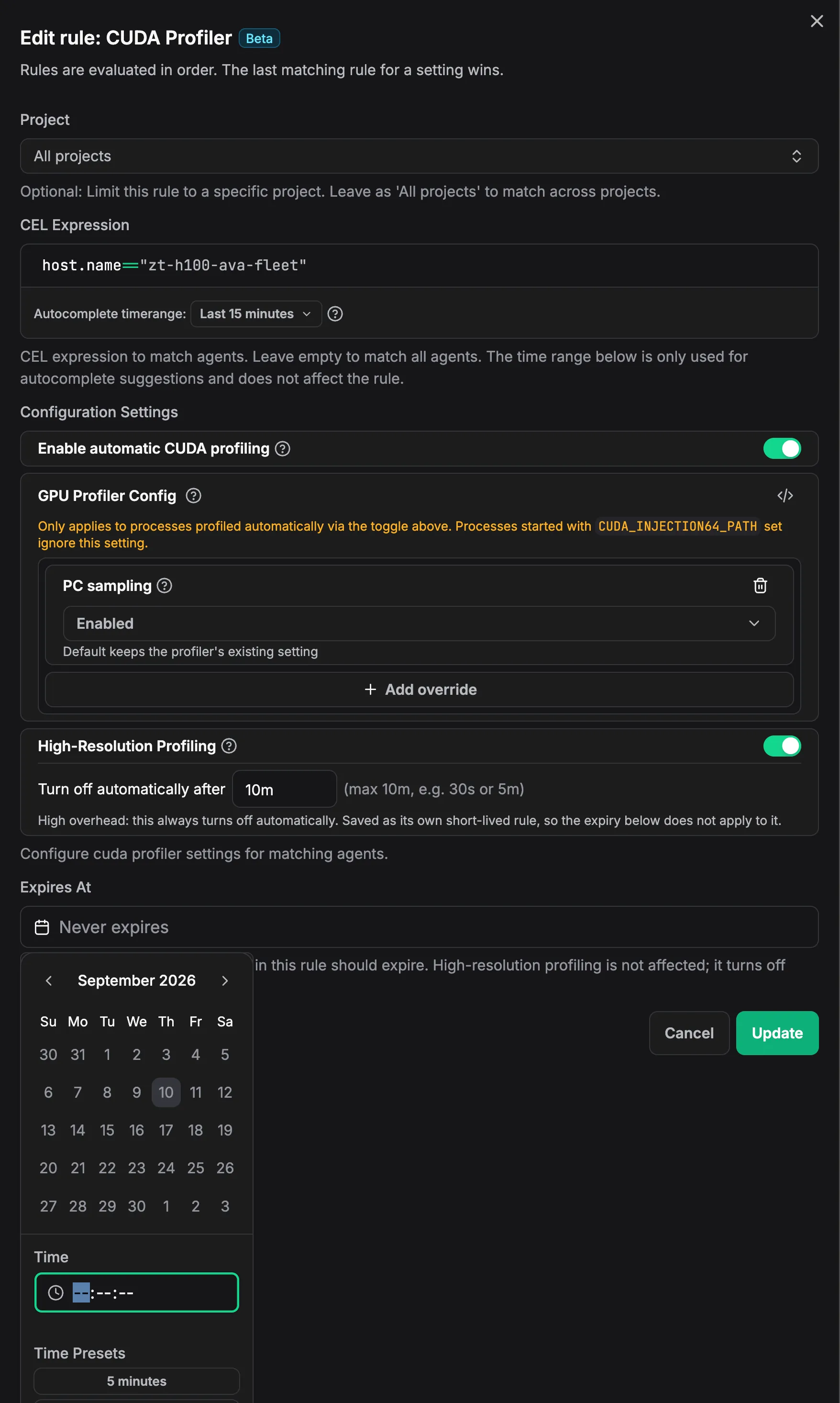
Enabling high-resolution profiling in a CUDA profiler rule. A CEL expression scopes it to matching agents, and the session turns itself off after the configured duration.
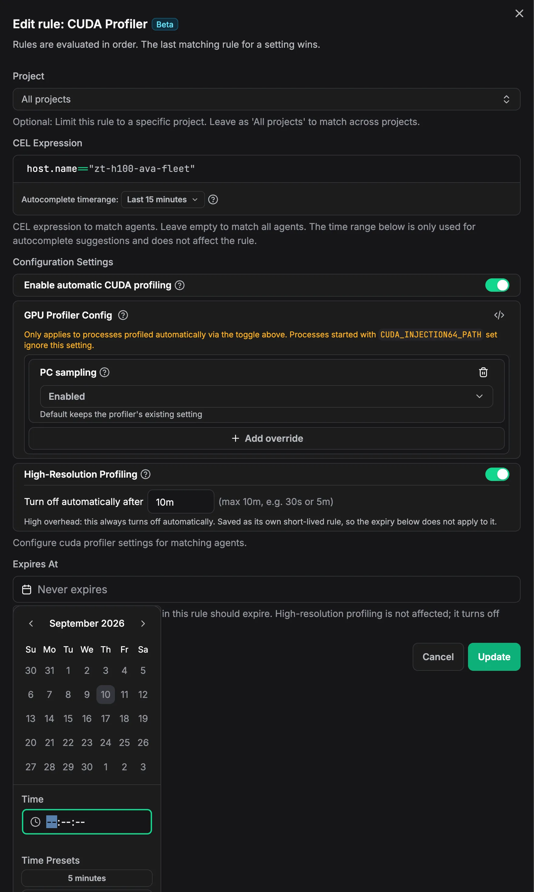
High-resolution profiling has noticeably more overhead than continuous sampled profiling, so it is intended for focused investigations rather than for staying on. The rule expires on its own; nothing has to be turned off afterward.
Once a session has run, the density strip above the timeline shows where high-resolution data exists within the selected time range, and the same workload filters as the flamegraph apply.
Zymtrace takes a different approach to working with GPU traces: no report files to manage, microsecond kernels that stay visible when zoomed out, and event timing shown alongside CPU launch stacks and GPU memory activity.
Large traces, no report files
The conventional workflow for per-kernel tracing produces a report file that you collect, move, and open in a separate viewer. That adds file handling to an investigation that already involves collecting and interpreting substantial amounts of data.
Zymtrace streams events directly into the timeline in a single request and renders chunks as they arrive. The first spans appear within a second, progress is reported against the expected event count, and you can pan and zoom while loading continues, up to one million events per view.
No intermediate trace file is created, exported, or downloaded. Profiling and analysis stay in the same UI, and the capture lands in the deployment you already run.
The timeline uses the same Rust, WebAssembly, and WebGL renderer we built for the AI flamegraph. Incremental loading and GPU-accelerated rendering keep navigation responsive as you move from the execution overview down to individual operations.
Microsecond kernels stay visible
At wider zoom levels, microsecond kernels become narrower than one pixel. Dropping those spans, which is what culling by width amounts to, can make an active stream appear empty.
Zymtrace preserves them with two rendering layers:
- A green leaf indicator places a minimum-width marker in every pixel column that holds a leaf span, including events recorded with zero duration.
- Density shading accumulates span coverage within each physical pixel column. Opacity reflects how much of the column is covered, and color reflects the dominant contributor, so a dense region reads as a miniature of the spans underneath it rather than a flat haze.
Repeated launch groups, gaps, and changes in activity therefore remain visible before individual events can be resolved. You can locate a region worth investigating without first zooming in far enough to see every kernel.
Timing, stacks, and memory
Each kernel launch, memory copy, and synchronization event is recorded individually with nanosecond timestamps. That preserves the detail needed to measure microsecond-scale launch gaps, inspect copy ordering, and compare repeated sequences.
Each CUDA stream has its own lane. Synchronization calls appear on adjacent (sync) lanes, so stream-synchronize and event-synchronize spans sit next to the kernels they wait on instead of covering them. Device-wide synchronizations collect in a No stream (sync) lane, and NVTX ranges emitted by the workload appear as their own rows (see Introducing NVTX Support in Zymtrace).
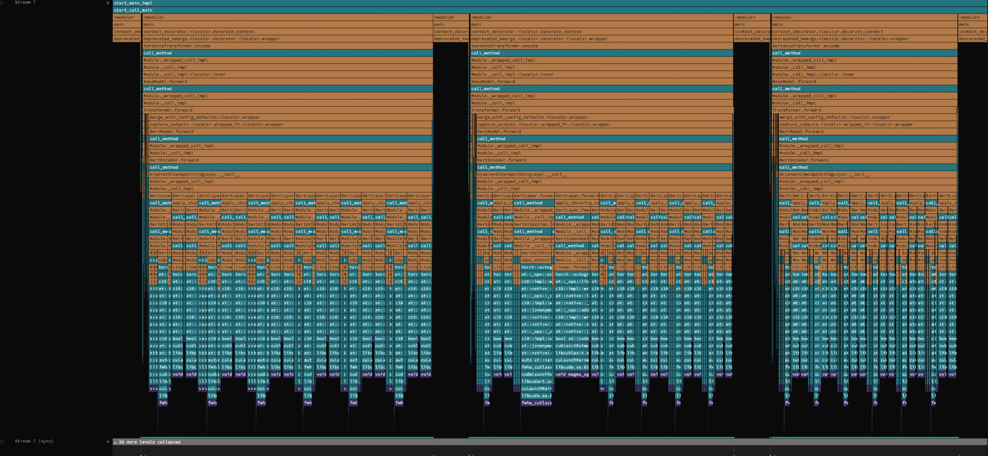
Every span carries its full CPU launch stack, from the application module through the framework and native code down to the launch call. Expanding a stream renders that hierarchy above the kernels, which is what distinguishes two application paths that launch the same kernel. Collapsed lanes show only the leaf frames, with N more levels collapsed marking what is hidden. Hovering a span gives the kernel name, duration, memcpy direction (H2D, D2H, D2D), and the launching thread.
The GPU Memory track under the stream lanes aligns allocation changes with execution, so memory growth can be investigated alongside the operations next to it and the code paths that issued them.
Navigation is direct: ctrl+drag zooms to a selection, right click zooms back out, click zooms onto a span, shift+scroll pans, and span names are searchable by regex. The language and sub-kind filters are the ones the flamegraph legend already uses.
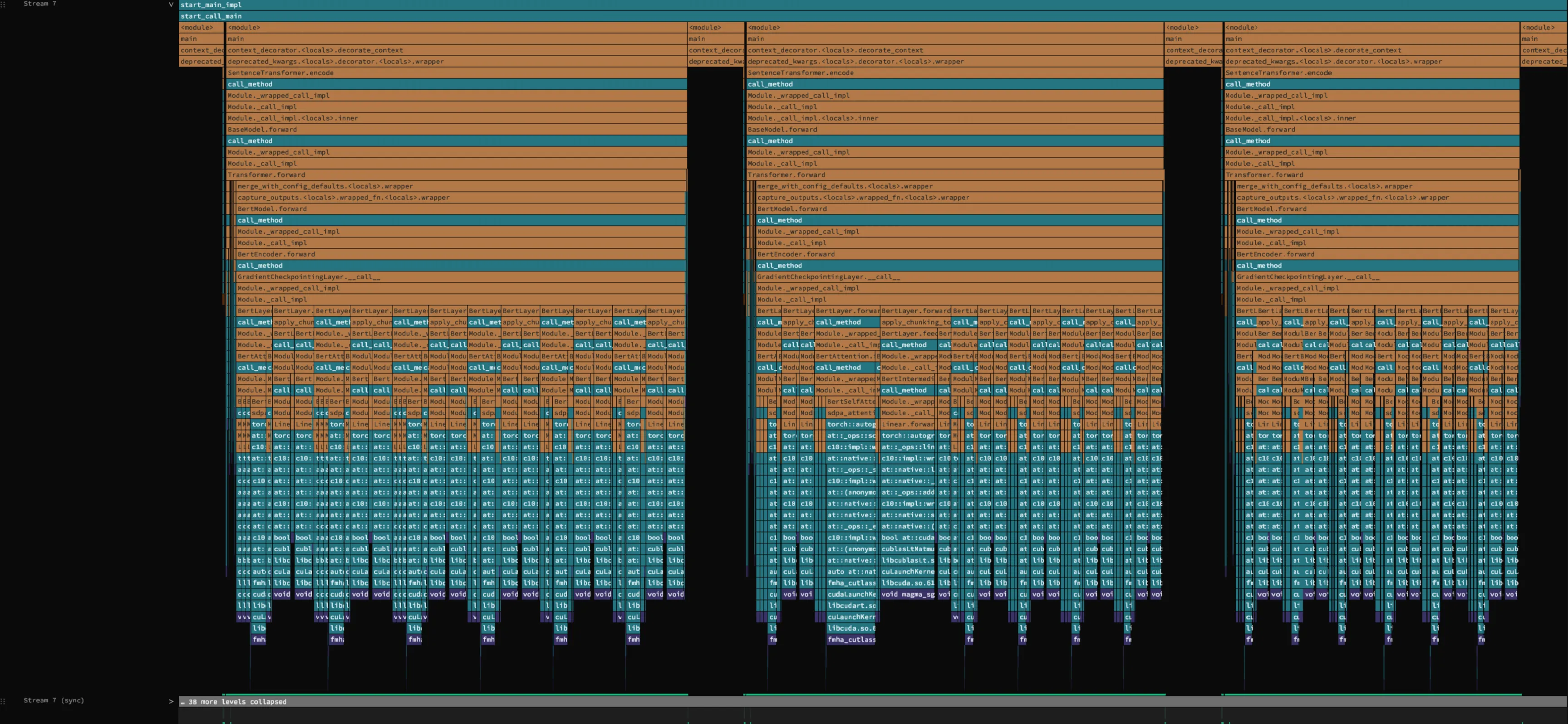
Three batches on one expanded stream lane. The Python stack sits above the kernels, and the idle gaps between batches are part of the picture.
An embedding workload: 568 seconds to 82 seconds
The workload used sentence-transformers to embed roughly 500,000 text passages. The baseline ran model.encode with fp32, batch size 64, and inputs copied from pageable host memory. Each batch issued 98 CUDA launches through six BERT layers.
We checked embeddings against the baseline after each change. Mean cosine similarity remained at or above 0.999999 in this test.
1. Reduce gaps between batches
At batch boundaries, a launch group ended, the stream went idle, then three host-to-device copies appeared, each followed by a synchronization, before the next group began.
Gaps ranged from 8ms to 75ms, against launch groups of around 55ms. The launch stacks connected the copies to the tokenizer’s output tensors, input_ids, token_type_ids, and attention_mask, each moved to the GPU separately by at::native::copy_impl through cudaMemcpyAsync. The synchronization after each copy follows from the host buffers being pageable: the CPU waits for one copy to finish before issuing the next.

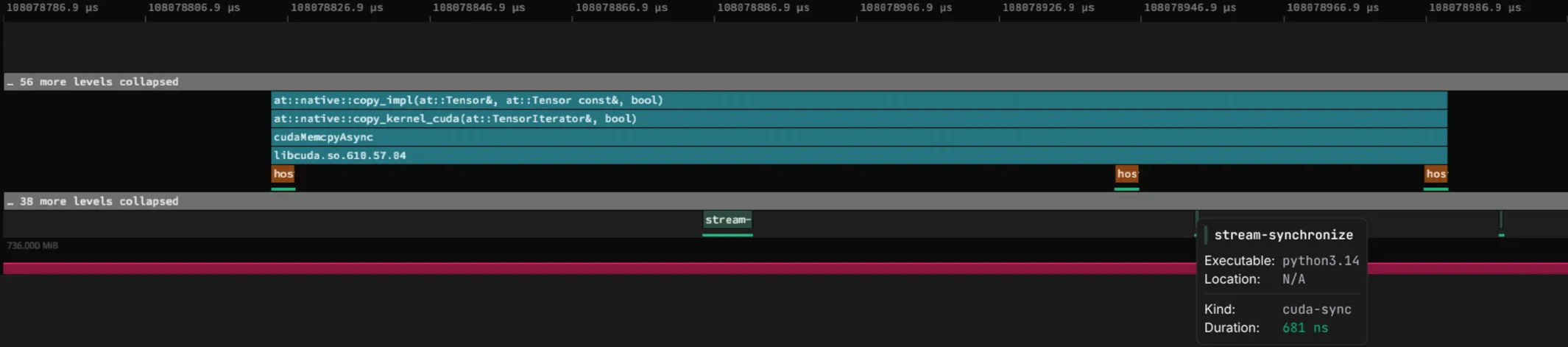
A batch boundary: an idle stream, three host-to-device copies with a synchronization after each, then the next launch group. The highlighted synchronization took 7 µs.

The gap itself is host time, so the change was on the host side: prefetch tokenization for the next batch while the GPU processes the current one, and shorten Python’s GIL switch interval so the launching thread regains the interpreter sooner. Typical gaps fell from around 20ms to 6ms, reducing run time from 568s to 479s.
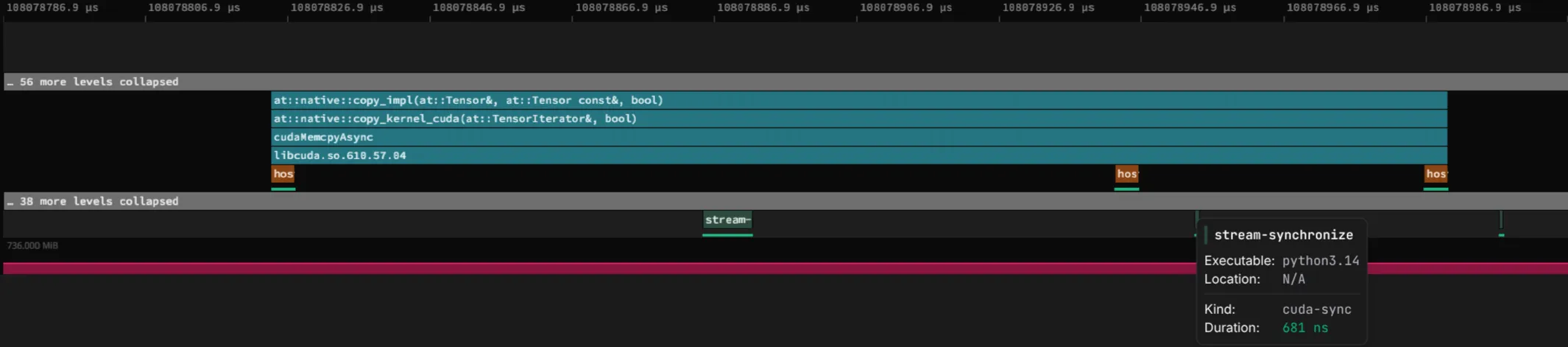
Start of a batch. The three copies appear with their launch stack, with synchronization calls on the sync lane between them.
2. Switch matrix multiplication to fp16
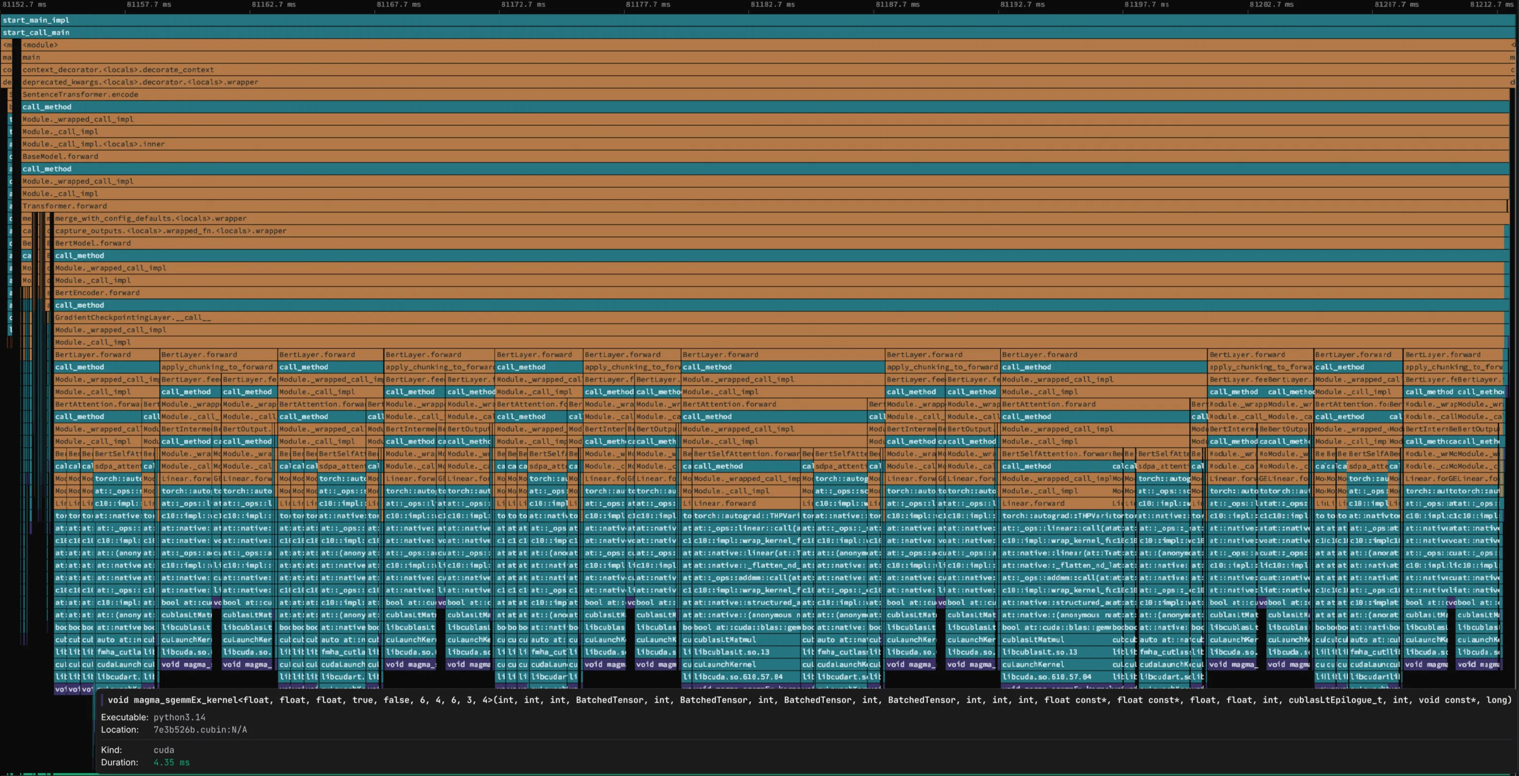
Expanding a batch showed six repeated BertLayer.forward calls, with fp32 sgemm kernels dominating each layer. The flamegraph had already identified sgemm as the largest contributor; the timeline added its placement and repetition within each batch.
Switching to fp16 with model.half() reduced run time from 479s to 143s, the average batch duration from around 75ms to 14ms, and the gap between batches from 6ms to 2ms.
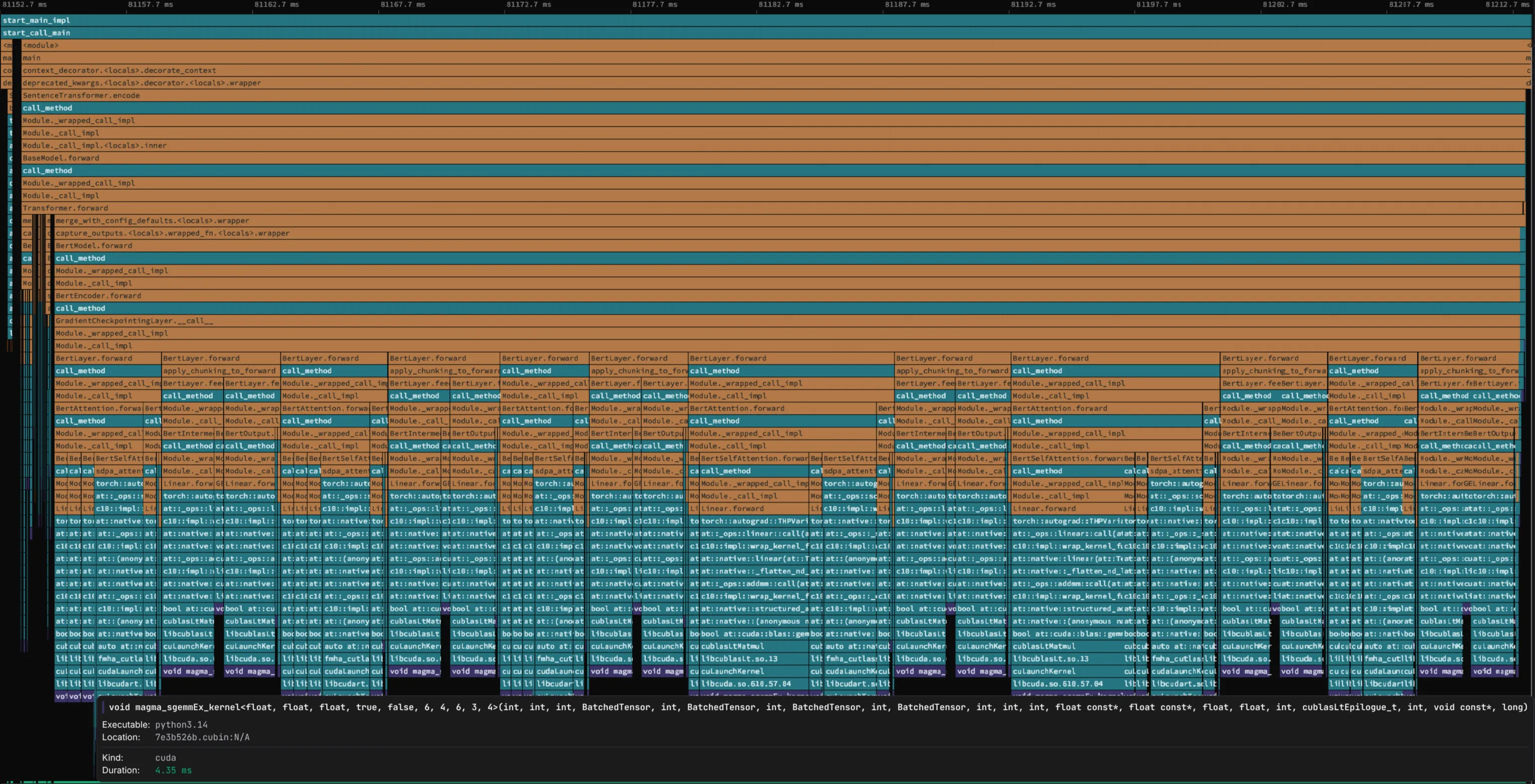
One batch, stream lane expanded. Six BertLayer.forward frames under BertEncoder.forward, sgemm and fmha kernels at the bottom.
3. Increase batch size
With shorter kernels, sub-millisecond gaps at batch starts became more apparent: launch latency was no longer hidden behind kernel duration, so the gaps around each kernel made up a larger share of the run. A batch-size sweep led us to increase the batch size from 64 to 128, bringing run time down to 136s.
4. Batch by token length
Searching for fmha.* identified the attention kernels, six per batch, one per layer. Comparing instances across the trace showed longer durations toward the middle of the run and shorter durations toward the end.
The inputs had been sorted by character count, which did not consistently group passages by token count. Some batches mixed short and long token sequences, and attention is quadratic in the padded sequence length, so those batches paid for their longest member.
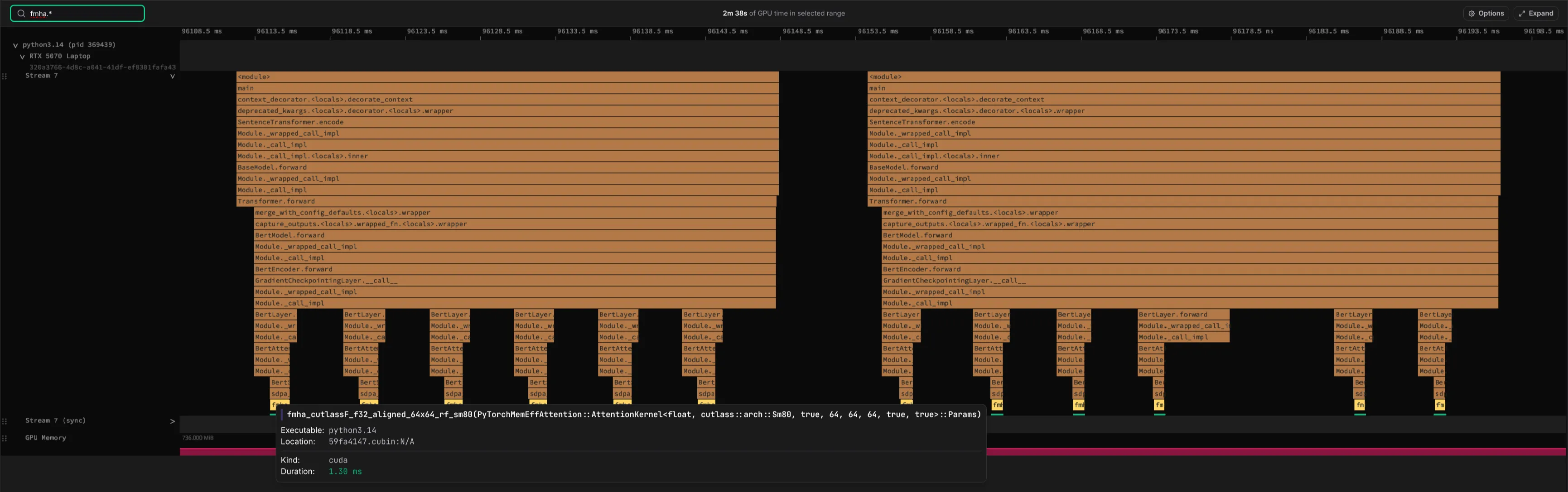
Searching for fmha across two batches. Six hits per batch, one per layer, each with its duration on hover.
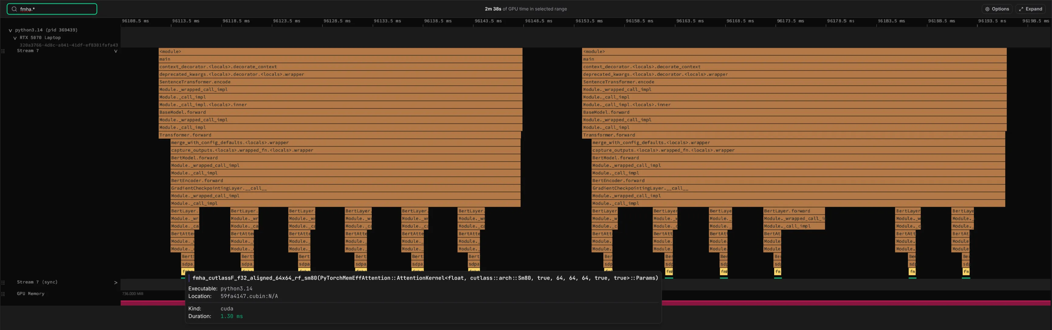
Batching by actual token length reduced run time from 136s to 82s. The useful evidence was the variation between kernel instances across the run, which aggregate kernel time does not expose.
Summary
| Observation | Change | Run time | Passages/s |
|---|---|---|---|
| baseline | fp32, batch size 64 | 568s | 853 |
repeated inter-batch gaps of ~20ms | prefetch tokenization, sys.setswitchinterval | 479s | 1050 |
fp32 sgemm dominated the layers | model.half() | 143s | 3484 |
| sub-millisecond launch gaps at batch start | batch size 128 | 136s | 3685 |
| attention duration varied across the run | batch on token length | 82s | 6100 |
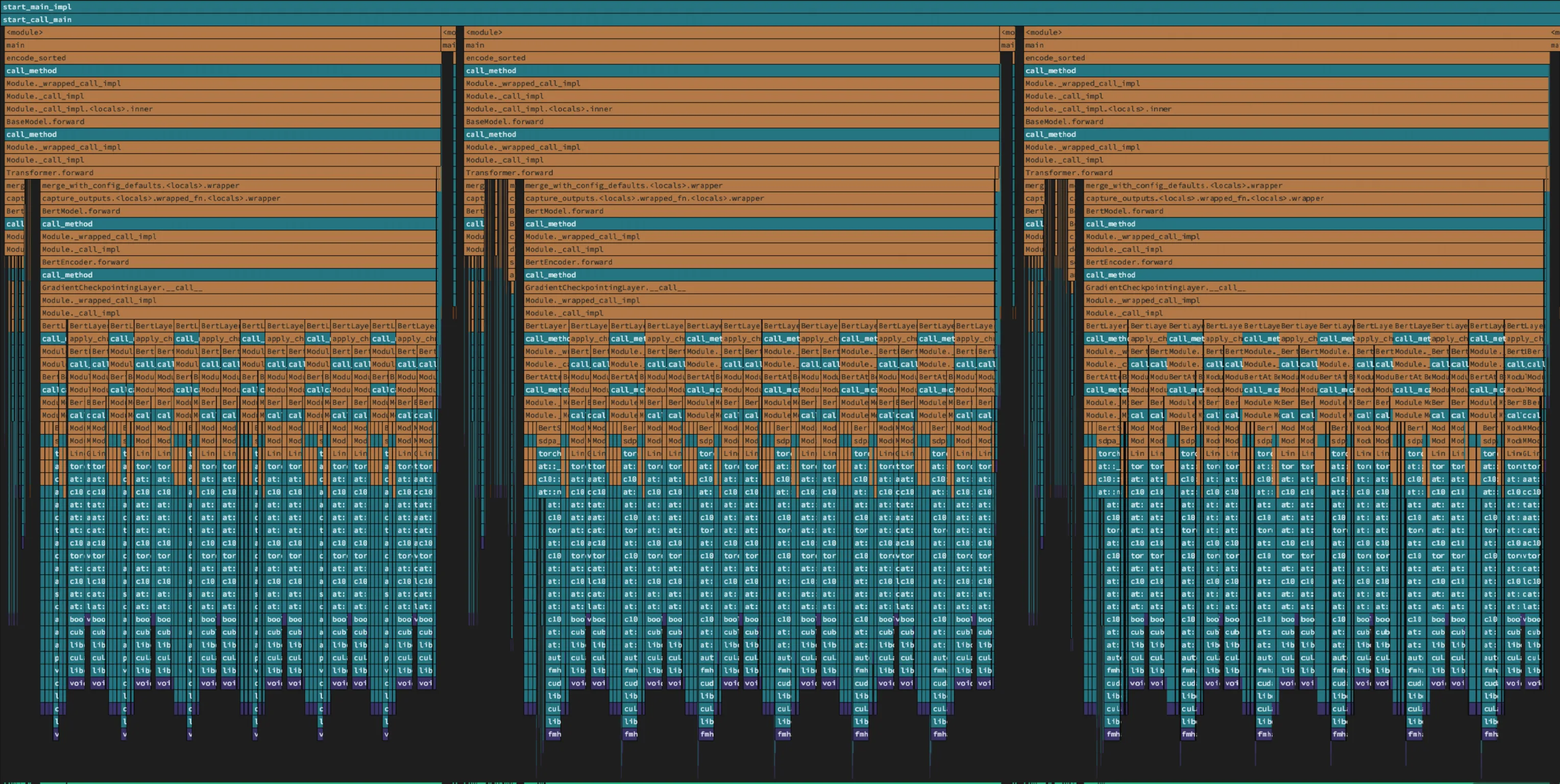
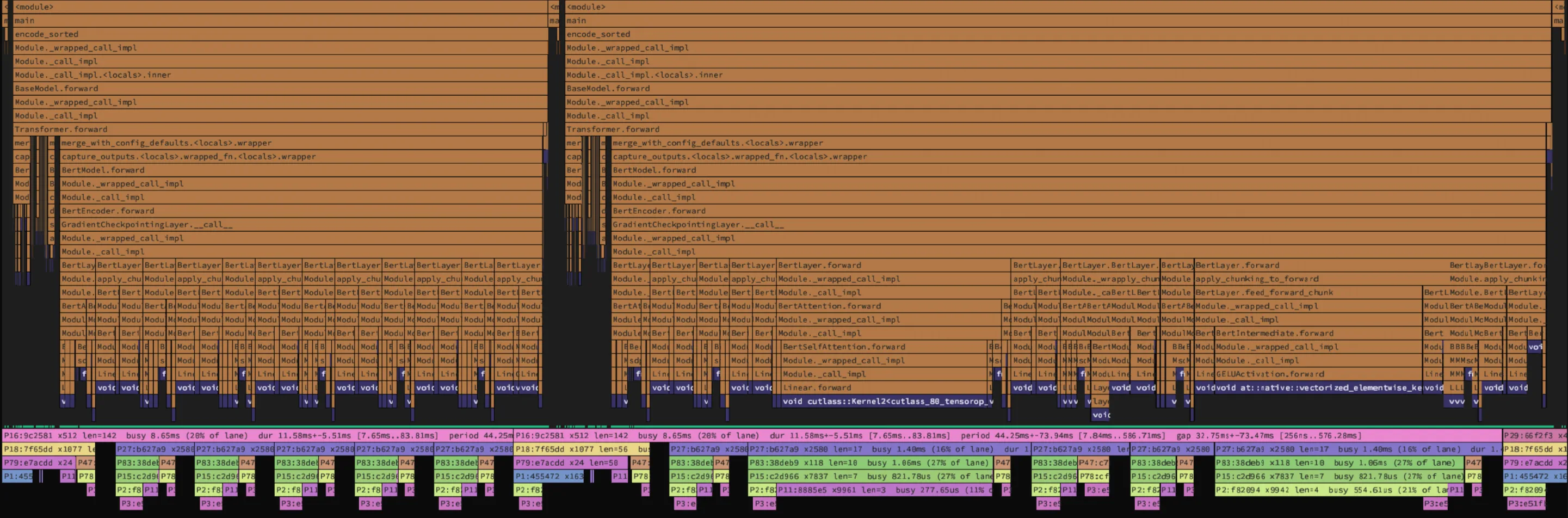
Together, these changes produced a 6.9x speedup on this workload. Below is the same view as the overview above, after the changes: three batches, launch groups packed back to back, the gaps between them nearly gone.
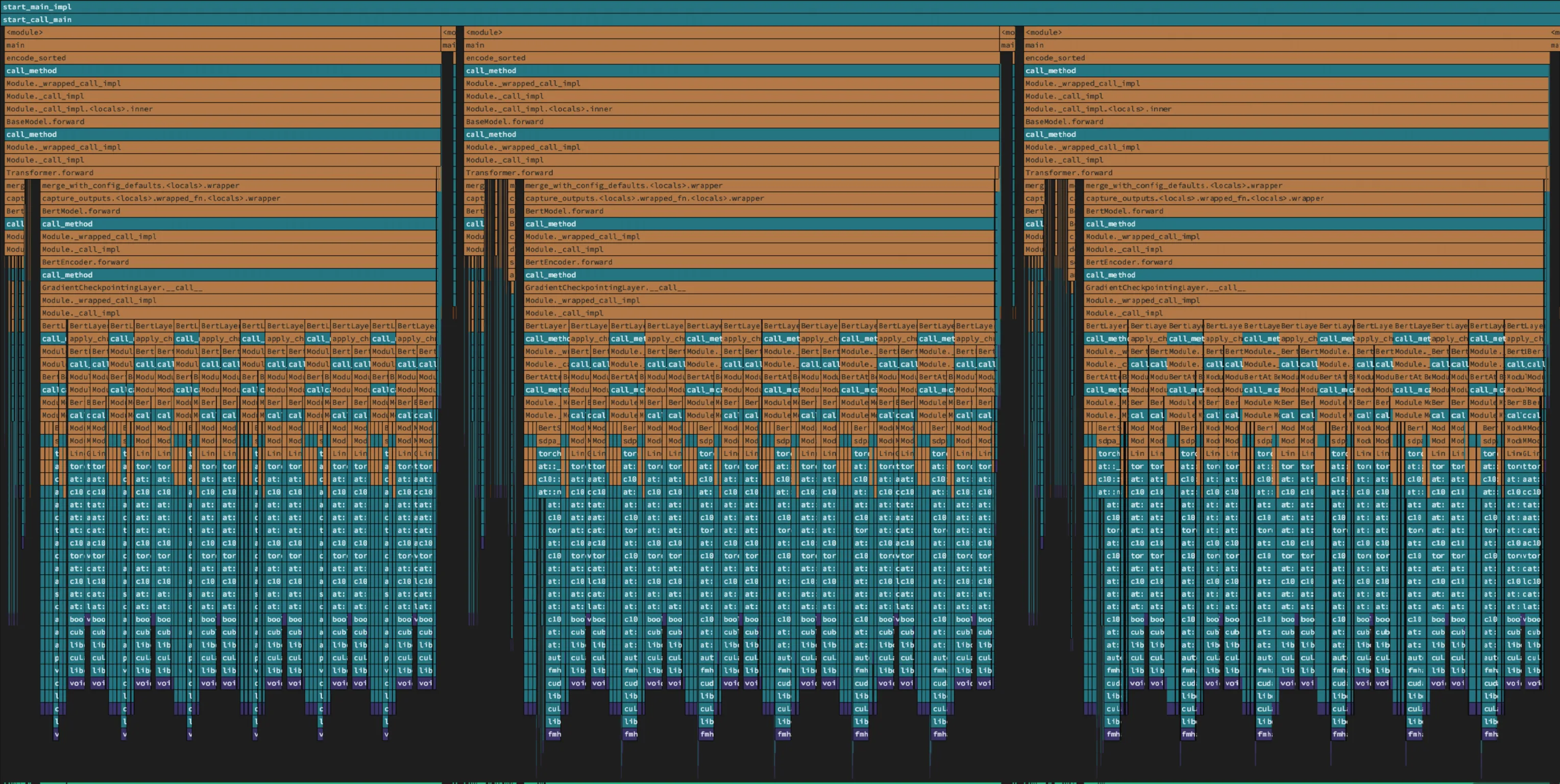
Three batches after the changes, with the stream lane expanded. The same six-layer shape remains, with gaps between batches nearly gone. In this window, a batch that took 47 ms in the baseline takes 12 ms.
Analyze execution patterns through MCP
The embedding investigation required repeated measurements of batch duration, inter-batch gaps, and attention-kernel duration. Collecting them by hand meant zooming, hovering, and copying values out of the trace.
The Zymtrace MCP server exposes the same measurements as tools. timeline_density locates where high-resolution data exists in a scope and how much of it there is; timeline_patterns detects repeated launch patterns in one window and reports them per lane. Coverage spans individual operations and repeated event sequences, including launch groups and NVTX-delimited layers, with occurrence counts, duration and spread, repetition period, gaps, and busy time as a share of the lane. Patterns nest, so a batch, the layers inside it, and the kernel groups inside those are all addressable, and a per-occurrence mode returns every instance’s extents for drift analysis.
Agents can compare pattern instances across a trace, identify where timing changes, and combine those findings with CPU and GPU flamegraphs, host and GPU metrics, and inference-engine metrics available through the same server (see Zymtrace Agent Skills). For this workload, that means measuring how batch intervals change, comparing attention-kernel durations across the run, and quantifying the effect of each optimization without manually sampling individual events.
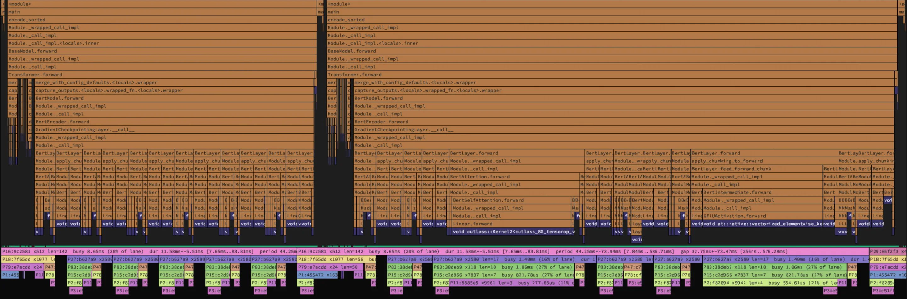
Detected patterns for the embedding workload, drawn as tracks under the stream lane. The batch pattern on top, layers and kernel groups nested below, each with count, busy share, duration and spread, period, and gap. The MCP tool returns the same data as text.
Appendix: when to use a flamegraph or a timeline
A GPU flamegraph aggregates profiling data across a selected period, grouping it by kernel and originating CPU stack. Width represents the selected profiling metric, not elapsed time, and adjacent frames need not have executed consecutively.
Use it to prioritize optimization: identify dominant kernels, trace them to application code, and inspect stall reasons or instruction-level behavior where available.
A timeline preserves individual events in execution order. Horizontal position represents time and span width represents duration, and separate stream lanes reveal concurrency, overlap, and gaps.
Use it when the performance question depends on the relationship between operations.
| Question | View |
|---|---|
| Which kernels and application code paths dominate GPU activity? | GPU flamegraph |
| Which stall reasons or instructions warrant investigation? | GPU flamegraph with the relevant profiling data |
| Where do gaps appear between launches? | Timeline |
| Are transfers overlapping with compute? | Timeline |
| Where do synchronization calls occur relative to GPU execution? | Timeline |
| How do kernel durations and batch intervals change across a run? | Timeline |
| What executes around a GPU memory increase? | Timeline with the memory overlay |
Both views carry CPU launch stacks. In the embedding example, the flamegraph identified sgemm as the dominant kernel, while the timeline exposed the inter-batch gaps and the variation in attention-kernel duration.
Two boundaries are worth keeping in mind. An empty interval on one stream does not establish that the entire GPU was idle, so check the other lanes. And the timeline shows that a gap exists and what borders it, not what the CPU was doing inside it; for that, read the CPU profile over the same window.
Sounds interesting?
The GPU execution timeline is available now in the CUDA profiles view, in beta. It uses the same profiler injection you already have; high-resolution profiling is switched on from the UI when you need it.
Get started today at no cost. You can host Zymtrace wherever you want. We provide both Helm charts and Docker Compose configs, so if you are familiar with either, you can have it running in minutes.
Once deployed, the profiling agent continuously profiles running processes on your machines with low overhead. No code changes, no instrumentation required. Profiles for running applications appear automatically in the Zymtrace UI.
For GPU profiling, Zymtrace supports CUDA workloads, including those built with frameworks like PyTorch and JAX. For CPU profiling, Zymtrace supports major languages out of the box, including Python, Java, Kotlin, Node.js, PHP, Ruby, .NET, C/C++, Rust, Go, and more.


